Determining Model Parameter Sensitivity Using Sensitivity Analysis
Sensitivity analysis quantifies the impact of various factors on a model’s output. When a model has multiple undetermined parameters, these parameters can be analyzed to identify key parameters that significantly affect the model’s results. Targeting these highly sensitive parameters for identification can effectively improve the model’s accuracy and reliability, especially for complex models with numerous parameters.
Main Sensitivity Analysis Methods
Local Sensitivity Analysis
Local sensitivity analysis focuses on the impact of small changes in input parameters around a specific point on the model output. It is usually achieved by calculating partial derivatives or making small perturbations near the parameter values. Examples include the One-At-a-Time (OAT) method and the differential method (calculating partial derivatives). These methods are computationally simple and suitable for quickly understanding the local response characteristics of the model to individual parameters.
$$ S_i^{\text{OAT}} \approx \frac{y(x_1, …, x_i+\Delta x_i, …, x_n) - y(x_1, …, x_i, …, x_n)}{\Delta x_i} $$
- Advantages: Low computational cost, easy to implement.
- Disadvantages: Only reflects the local impact of parameters at a specific point, cannot reveal the effect of parameter changes over their entire range, and ignores interactions between parameters.
- Suitable for simple models with limited parameter variation ranges, to quickly understand the local response characteristics of the model to individual parameters.
Global Sensitivity Analysis
Global sensitivity analysis examines the impact of input parameters varying over their entire range of values on the model output. It can capture non-linear relationships and interactions between parameters, providing a more comprehensive sensitivity assessment.
Morris Method
The Morris method involves a series of designed “elementary effects” perturbations in the parameter space. It calculates the mean effect and standard deviation for each parameter, thereby distinguishing the overall impact of parameters from non-linear or interaction effects.
- Advantages: Computational cost is linearly related to the number of parameters, making it relatively efficient and suitable for high-dimensional parameter spaces. It can quickly screen out important parameters.
- Disadvantages: Results are mainly used for qualitative ranking and are generally not suitable for precise quantitative analysis.
The specific steps are as follows:
First, calculate the elementary effect:
$$ EE_i = \frac{y(x_1, …, x_i + \Delta, …, x_k) - y(x_1, …, x_i, …, x_k)}{\Delta} $$
where $\Delta$ is the perturbation step size for the parameter, and $i=1,2,\ldots,k$ denotes the $i$ -th parameter. For each parameter $i$, multiple elementary effects $EE_i^{(r)}$ are calculated along $R$ different sampling paths, $r=1,2,\ldots,R$.
Next, calculate the mean, which measures the average effect of the parameter:
$$ \mu_i = \frac{1}{R} \sum_{r=1}^R EE_i^{(r)} $$
Since elementary effects in non-monotonic functions can cancel each other out (positive and negative values), the mean of absolute values is often used:
$$ \mu_i^* = \frac{1}{R} \sum_{r=1}^R |EE_i^{(r)}| $$
Simultaneously, calculate the standard deviation, which reflects the non-linearity and interaction effects of the parameter:
$$ \sigma_i = \sqrt{\frac{1}{R-1} \sum_{r=1}^R \left(EE_i^{(r)} - \mu_i\right)^2} $$
A larger $\mu_i^*$ indicates that parameter $x_i$ has a more significant impact on the model output. A larger $\sigma_i$ suggests that the effect of this parameter has strong non-linearity or interacts significantly with other parameters.
For specific methods and implementation details, refer to this documentation. Note the following:
- Standardize the model inputs and outputs to be dimensionless to ensure the comparability of sensitivity results.
- The Morris method relies on special sampling designs, common ones being Trajectory Design and Radial OAT Design.
- Scatter plots in the $\sigma_i$ - $\mu_i^*$ plane can be used to visually distinguish important parameters from non-important ones.
Sobol Method
The Sobol method is based on variance decomposition. It decomposes the total variance of the model output into contributions from individual input parameters and their interactions. This allows for the quantitative assessment of the main effect and total effect sensitivity indices for each parameter.
- Advantages: Rigorous theoretical basis, capable of comprehensively capturing linear, non-linear, and multi-parameter interaction effects, providing precise quantitative sensitivity indicators.
- Disadvantages: Computationally intensive, usually requiring a large number of model runs and samples, leading to high computational costs.
The total variance of the model output is:
$$ V = \mathrm{Var}[Y(\mathbf{X})] $$
where $\mathbf{X} = (X_1, X_2, …, X_k)$ is the input parameter vector, and $Y$ is the model output.
The first-order Sobol index (main effect sensitivity index) is defined as:
$$ S_i = \frac{V_i}{V} = \frac{\mathrm{Var}{X_i} \left( \mathbb{E}{\mathbf{X}_{\sim i}}[Y | X_i] \right)}{V} $$
where $V_i$ is the contribution of parameter $X_i$ alone to the output variance, and $\mathbf{X}_{\sim i}$ represents all parameters except $X_i$.
The total Sobol index (total effect sensitivity index) is defined as:
$$ S_{T_i} = 1 - \frac{V_{\sim i}}{V} = \frac{\mathbb{E}{\mathbf{X}{\sim i}} \left( \mathrm{Var}{X_i}[Y | \mathbf{X}{\sim i}] \right)}{V} $$
where $V_{\sim i}$ is the variance contribution of all parameters except $X_i$. $S_{T_i}$ measures the total contribution of parameter $X_i$ and all its interactions with other parameters to the output.
Sobol indices are typically calculated using Monte Carlo sampling, where appropriately designed sample matrices are used to estimate the above variance components.
FAST Method (Fourier Amplitude Sensitivity Test)
The FAST method utilizes the principles of Fourier transforms. It maps the multi-dimensional parameter space to a one-dimensional frequency space and analyzes the spectral components of the model output to calculate parameter sensitivities, thereby improving the efficiency of sensitivity calculations.
- Advantages: Relatively high computational efficiency, suitable for medium-dimensional parameter spaces, and can estimate parameter sensitivity indices relatively quickly.
- Disadvantages: Limited ability to capture highly non-linear and higher-order parameter interactions, and sensitivity results may not be sufficiently precise.
- Suitable for models where the input-output relationship is relatively smooth or approximately linear.
Each input parameter $X_i$ is associated with a different frequency $w_i$ as a parameter of a sinusoidal function, constructing a single-variable function in the parameter space:
$$ X_i = G_i(\omega s) = \frac{1}{2} + \frac{1}{\pi} \arcsin(\sin(\omega_i s)) $$
where $s$ is a one-dimensional frequency parameter, and $\omega_i$ is the frequency chosen for parameter $X_i$.
The model output $Y$ varies with $s$, forming a one-dimensional function:
$$ Y(s) = f(X_1(s), X_2(s), …, X_k(s)) $$
By performing a Fourier transform on $Y(s)$ and calculating the amplitudes of different frequency components, the sensitivity index $S_i$ for parameter $X_i$ is calculated from the variance contribution of the corresponding frequency component:
$$ S_i = \frac{\sum_{m=1}^\infty \left( A_{im}^2 + B_{im}^2 \right)}{\mathrm{Var}[Y]} $$
where $A_{im}$ and $B_{im}$ are the cosine and sine coefficients of the Fourier series corresponding to the frequency $m \omega_i$.
Case Study: Analyzing Geometric Parameter Sensitivity of Lithium-Ion Battery SPMe Model using Sobol Method
Several projects and discussions have mentioned parameter sensitivity analysis in PyBaMM, such as Mrzhang-hub/pybamm-param-sensitivities and Questions on checking sensitivities. However, these works primarily focus on the sensitivity analysis of electrochemical and material parameters, with little attention to geometric parameters (e.g., electrode thickness, separator thickness, particle radius). This is mainly because the sensitivity analysis of geometric parameters involves changes in mesh generation and solvers. This case study uses the Sobol method to analyze the sensitivity of geometric parameters in the Single Particle Model with electrolyte (SPMe) for lithium-ion batteries. The main tools used are pybamm (for battery modeling and simulation) and salib (for sensitivity analysis). The project repository is Mingzefei/battery_model_sensitivity_analysis.
Core Libraries
- PyBaMM (Python Battery Mathematical Modelling): An open-source Python battery modeling package that supports various models like DFN, SPM, and SPMe. PyBaMM provides a flexible framework for simulating battery behavior, parameter estimation, and experimental design, enabling rapid construction and solution of complex electrochemical and thermophysical models.
- SALib (Sensitivity Analysis Library in Python): A Python library for sensitivity analysis, offering methods like Sobol, Morris, and FAST. SALib helps understand how model outputs are sensitive to changes in input parameters, identify key parameters and their interactions, and can be used for quantifying uncertainty and ranking the importance of model parameters.
Code Implementation
This project is based on PyBaMM’s SPMe (Single Particle Model with Electrolyte) model. Typical geometric parameters such as positive electrode thickness, negative electrode thickness, and separator thickness were selected. The Sobol method from SALib was used for global sensitivity analysis. The specific implementation can be found in battery_model_sensitivity_analysis/notebooks/spme_geometric_sobol_analysis.ipynb.
Quantifying Time Series Differences
The output of the SPMe model (e.g., voltage) is time-series data. Sensitivity analysis requires quantifying the difference between the output curve $Y(t)$ after parameter changes and the baseline curve $Y_b(t)$. This is considered from the following perspectives:
-
Position Difference ($\delta_p$): Measures the overall positional shift.
$$ \delta_p[Y(t), Y_b(t)] = \text{mean}[Y(t)] - \text{mean}[Y_b(t)] $$
-
Scale Difference ($\delta_s$): Measures the difference in amplitude.
$$ \delta_s[Y(t), Y_b(t)] = (\max[Y(t)] - \min[Y(t)]) - (\max[Y_b(t)] - \min[Y_b(t)]) $$
-
Shape Difference ($\delta_r$): Measures the shape difference after correcting for position and scale. In this study, we use the Root Mean Square Error (RMSE) to quantify the shape difference:
$$ \delta_r[Y(t), Y_b(t)] = \text{RMSE}(Y(t), Y_b(t)) = \sqrt{\frac{1}{M} \sum_{i=1}^{M} (Y(t_i) - Y_b(t_i))^2} $$
where $M$ is the number of evaluation time points.
This project will use a combined difference metric $\Delta_i = \delta_p + \delta_s + \delta_r$ as a single measure to quantify the overall difference between the voltage curve $V(t)$ and the baseline voltage curve $V_b(t)$. This metric will serve as the target function output for the Sobol analysis.
   import numpy as np

   def calculate_combined_difference(Y, Y_b):
      # Position difference
      delta_p = np.mean(Y) - np.mean(Y_b)

      # Scale difference
      delta_s = (np.max(Y) - np.min(Y)) - (np.max(Y_b) - np.min(Y_b))

      # Shape difference - RMSE
      delta_r = np.sqrt(np.mean((np.array(Y) - np.array(Y_b))**2)) # Ensure Y, Y_b are numpy arrays

      # Combined difference
      Delta_i = delta_p + delta_s + delta_r
      return Delta_i
Parameter Selection and Range Setting
Key geometric parameters in the SPMe model (e.g., positive electrode thickness, negative electrode thickness, separator thickness) are selected, and reasonable physical value ranges are set for each parameter.
   param_definitions = {
      "Negative electrode thickness [m]": {
         "default": default_param["Negative electrode thickness [m]"],
         "bounds_factor": 0.2,  # Variation +/- 20%
      },
      "Positive electrode thickness [m]": {
         "default": default_param["Positive electrode thickness [m]"],
         "bounds_factor": 0.2,
      },
      "Separator thickness [m]": {
         "default": default_param["Separator thickness [m]"],
         "bounds_factor": 0.2,
      },
      "Negative particle radius [m]": {
         "default": default_param["Negative particle radius [m]"],
         "bounds_factor": 0.2,
      },
      "Positive particle radius [m]": {
         "default": default_param["Positive particle radius [m]"],
         "bounds_factor": 0.2,
      },
   }

   problem = {
      "num_vars": len(param_definitions),
      "names": list(param_definitions.keys()),
      "bounds": [],
   }

   for name, props in param_definitions.items():
      lower_bound = props["default"] * (1 - props["bounds_factor"])
      upper_bound = props["default"] * (1 + props["bounds_factor"])
      problem["bounds"].append([lower_bound, upper_bound])
      print(
         f"Parameter: {name}, Default: {props['default']:.2e}, Bounds: [{lower_bound:.2e}, {upper_bound:.2e}]"
      )
Sampling and Simulation Solution
Using SALib’s sampling tools (e.g., Saltelli sampling), a large number of parameter combinations are generated within the parameter space. For each set of parameters, PyBaMM is called to run the SPMe simulation, and output indicators (e.g., terminal voltage, capacity during 1C constant current charge/discharge) are recorded.
   from SALib.sample import saltelli
   # import pybamm # Assuming pybamm is installed
   # import numpy as np # Assuming numpy is installed

   # Generate parameter samples
   # N is typically a power of 2, e.g., 1024. Total samples will be N * (D + 2) or N * (2D + 2)
   # D is the number of parameters (problem['num_vars'])
   param_values = saltelli.sample(problem, 1024)

   # Run a baseline simulation
   model_baseline = pybamm.lithium_ion.SPMe()
   param_baseline = pybamm.ParameterValues("Chen2020")
   experiment_baseline = pybamm.Experiment(["Discharge at 1C until 2.5 V"])
   sim_baseline = pybamm.Simulation(
      model_baseline, experiment=experiment_baseline, parameter_values=param_baseline
   )
   sol_baseline = sim_baseline.solve()
   t_eval_baseline = sol_baseline["Time [s]"].entries
   voltage_baseline = sol_baseline["Terminal voltage [V]"].entries

   # To ensure all simulations are compared at the same time points, define a fixed time vector t_eval_common
   # Use the maximum time from the baseline simulation and interpolate to 200 points
   max_time_baseline = t_eval_baseline[-1]
   t_eval_common = np.linspace(0, max_time_baseline, 200) # 200 evaluation points

   # Interpolate the baseline solution onto t_eval_common
   voltage_baseline_interp = np.interp(t_eval_common, t_eval_baseline, voltage_baseline)

   print(
      "Baseline simulation complete and common evaluation time points (t_eval_common) prepared."
   )
   print(f"Baseline simulation ran for {max_time_baseline:.2f} seconds.")
   print(
      f"Common evaluation time points range from {t_eval_common[0]:.2f}s to {t_eval_common[-1]:.2f}s with {len(t_eval_common)} points."
   )

   def evaluate_model_delta_i(parameter_sample):
      """
      Runs the PyBaMM SPMe model and calculates the combined difference metric Delta_i
      with the baseline voltage curve.
      Delta_i = delta_p + delta_s + delta_r
      where:
         delta_p: Position difference (mean_run - mean_baseline)
         delta_s: Scale difference ((max_run - min_run) - (max_baseline - min_baseline))
         delta_r: Shape difference (RMSE(run, baseline))
      Parameters:
         parameter_sample (np.array): Parameter sample generated by SALib.
      Returns:
         float: Combined difference metric Delta_i for the voltage curve.
      """
      model_run = pybamm.lithium_ion.SPMe()
      param_run = pybamm.ParameterValues("Chen2020") # Start with fresh default parameters each time

      current_params = {}
      for i, name in enumerate(problem["names"]):
         current_params[name] = parameter_sample[i]

      try:
         param_run.update(current_params)
         sim_run = pybamm.Simulation(
               model_run, experiment=experiment_baseline, parameter_values=param_run
         )
         sol_run = sim_run.solve(t_eval=t_eval_common)
         voltage_run = sol_run["Terminal voltage [V]"].entries

         if len(voltage_run) < len(t_eval_common):
               padding_value = (
                  voltage_run[-1]
                  if len(voltage_run) > 0
                  else param_run["Lower voltage cut-off [V]"]
               )
               voltage_run_padded = np.full_like(t_eval_common, padding_value)
               voltage_run_padded[: len(voltage_run)] = voltage_run
               voltage_run = voltage_run_padded

         # Calculate delta_p (Position difference)
         delta_p = np.mean(voltage_run) - np.mean(voltage_baseline_interp)

         # Calculate delta_s (Scale difference)
         range_run = np.max(voltage_run) - np.min(voltage_run)
         range_baseline = np.max(voltage_baseline_interp) - np.min(voltage_baseline_interp)
         delta_s = range_run - range_baseline

         # Calculate delta_r (Shape difference - RMSE)
         delta_r = np.sqrt(np.mean((voltage_run - voltage_baseline_interp) ** 2))

         # Calculate combined difference metric Delta_i
         # Note: Direct summation might lead to one term dominating due to different scales.
         # Weighting or normalization could be considered, but direct summation is used as per current requirement.
         delta_i = delta_p + delta_s + delta_r

         # print(f"Run with {current_params}, d_p={delta_p:.3f}, d_s={delta_s:.3f}, d_r={delta_r:.3f}, Delta_i={delta_i:.3f}")
         return delta_i

      except Exception as e:
         # print(f"Error during simulation with params {current_params}: {e}")
         return 1e6  # A large penalty value
Sensitivity Analysis
The simulation results are input into SALib’s Sobol analysis module to calculate sensitivity indicators such as the first-order Sobol index (main effect index) and total Sobol index (total effect index) for each parameter.
   from SALib.analyze import sobol

   # Perform Sobol analysis
   # Y_outputs should be the actual output results array from the previous simulation step
   # Note: Handle NaN values in Y_outputs if they can occur during simulation
   # Y_outputs_cleaned = Y_outputs[~np.isnan(Y_outputs)]
   # param_values_cleaned = param_values[~np.isnan(Y_outputs)]
   # If Y_outputs is cleaned, the corresponding param_values also need to be cleaned,
   # but this would break the Saltelli sample structure.
   # A better approach is to assign a reasonable penalty value for failed simulations
   # instead of NaN to maintain sample integrity.
   Si = sobol.analyze(problem, Y_outputs, calc_second_order=True, print_to_console=False)

   # Extract first-order and total effect indices
   S1_indices = Si['S1']
   ST_indices = Si['ST']

   print("First-order Sobol indices (S1):")
   for name, s1_val in zip(problem['names'], S1_indices):
      print(f"- {name}: {s1_val:.4f}")

   print("\\nTotal Sobol indices (ST):")
   for name, st_val in zip(problem['names'], ST_indices):
      print(f"- {name}: {st_val:.4f}")

   # If calc_second_order=True, second-order indices Si['S2'] and
   # corresponding parameter pairs Si['S2_conf'] can also be obtained.
Results Visualization
The final calculation results are shown in the figures below:
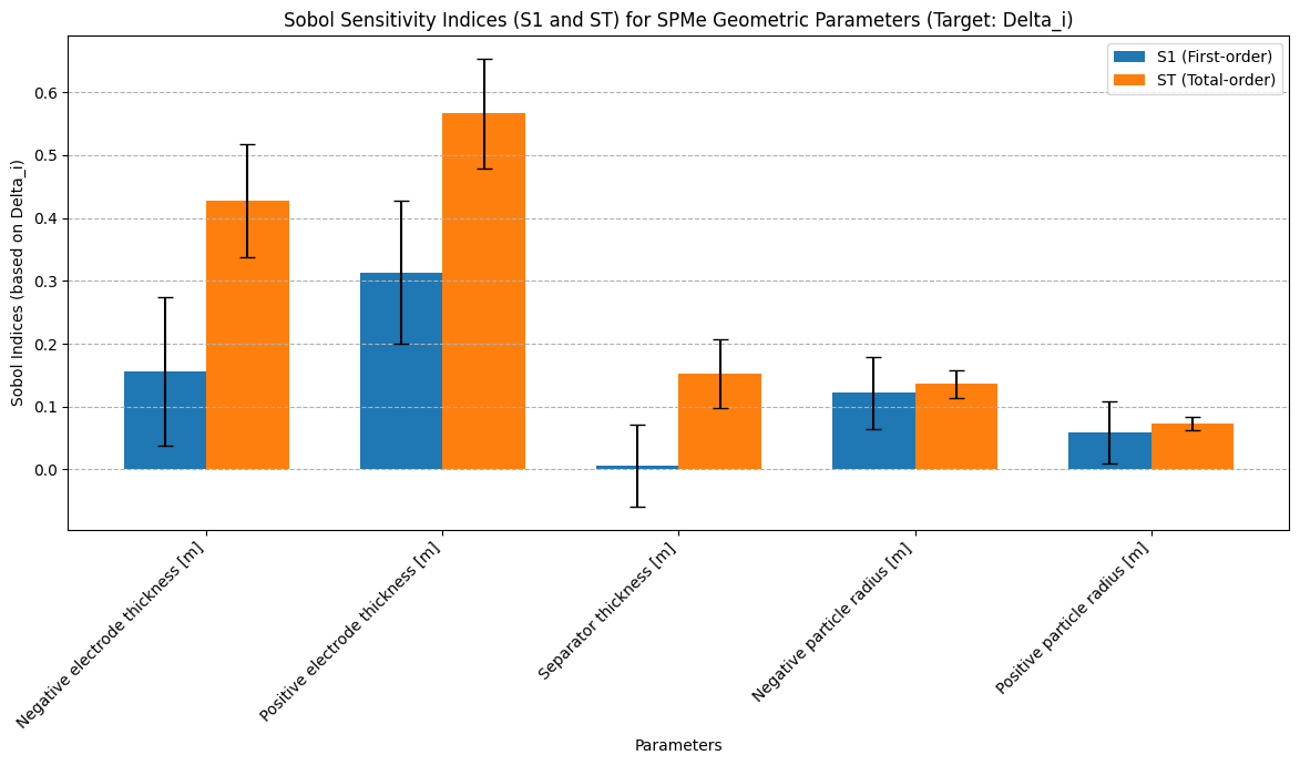
- Key Parameter Sensitivity: Some parameters (e.g.,
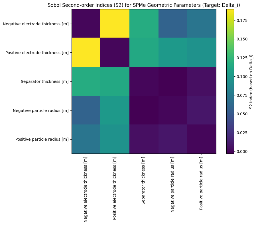
Positive electrode thickness,Negative electrode thickness) exhibit the highest S1 and ST values, indicating they have the most significant impact on the model output and are core factors requiring precise control in design and manufacturing. - Parameter Interaction Effects: The S2 heatmap shows strong S2 values between specific parameter pairs (e.g.,
Positive electrode thicknessandNegative electrode thickness), indicating significant interaction effects between these parameters.
Relevant literature also indicates that battery geometric parameters (especially electrode thickness) have a significant impact on key performance indicators such as capacity and power density.
- A Control-Oriented Simplified Single Particle Model with Grouped Parameter and Sensitivity Analysis for Lithium-Ion Batteries (2025) used Sobol sensitivity analysis to reduce the parameter set of SPM/SPMe from 9 to 6 highly sensitive parameters, with geometric parameters like electrode thickness among them.
- Global Sensitivity Methods for Design of Experiments in Lithium-ion Battery Context (2020) also confirmed the importance of geometric parameters in battery performance modeling and experimental design.
The above example can be further improved by increasing the number of parameters analyzed, refining the sampling range of parameters, increasing the number of samples, and optimizing the difference quantification method.